Looking at the means for the two data sets discussed in the “Measures of Centrality and Dispersion” article, we can compare the mean for set 1 (5.58) to that for set 2 (8.32). They are evidently different but how different? Another way of asking this question would be: how strong is the possibility that the two data sets (represented by their means) actually represent two different populations? Or, what is the likelihood that, despite the difference in means, the two data sets actually come from the same population. [In this context population means a group of subjects with a unique characteristic]. Another way of asking the question would be to establish an initial hypothesis – e.g., that the means for set 1 and set 2 are the same – which is called the Null Hypothesis: the means of both sets (populations) are the same¹.

A significance test is a statistical procedure that determines the degree to which observed data are consistent with a specific hypothesis about a population. Frequently, the significance is attributed a probability value – e.g., the probability that the observed data are consistent with the hypothesis is less than 5 in 100 which is the same as < 5%. This probability would be denoted by ‘p < 0.05’.

A confidence interval is the result of a statistical procedure which identifies the set of all plausible values of a specific parameter which are consistent with the observed data. A confidence interval includes all possible values of a parameter which, if tested as a specific null hypothesis (see above) would not lead us to conclude that the data contradict that particular null hypothesis.

Making some assumptions about the distribution of all possible values of the parameter (e.g., that the parameter data are normally distributed; a frequency distribution of all the data approximates a symmetrical  bell shape) we can relate statistical probability (p value) to confidence intervals. Although we cannot develop the theme fully here, accept that for normally distributed data the mean of the data ± 1.96 standard deviations of the mean (± 1.96*SD) divided by the square root of the number of data observations (Ön) includes 95% of all plausible values of the parameter. Thus, if the parameter value lies within the interval ± (1.96 SD/Ön) there is a ³ 95% probability that the value contradicts the hypothesis. For a more stringent test we might require that the parameter value mean resides within a 99% confidence interval which is ± 2.576 SD/Ön of the mean. In general, a narrow confidence interval indicates more precise information about the parameter value, whereas a broad interval indicates a greater degree of incertitude.

Comparing Means

To compare the means and test whether they are different, statistics provides a number of tests. Usually we start by stating a hypothesis, e.g., that the means are actually the same; we call this the Null Hypothesis. We then test the likelihood that the two means are the same and that the difference reported is simply due to random chance; we express this likelihood as a probability which ranges from 0 to 100% (0 to 1). If the probability that the means are different only because of random chance is very small (e.g., less than 5% (0.05)) then the likelihood that the means (and the populations from which they derive) are different is greater. In other words, we would reject the Null Hypothesis as untrue (or extremely unlikely).

Examples of statistical tests for comparing means include Student’s t test and simple Analysis of Variance (ANOVA). If we perform a Student’s t test on the data sets  from and test the Null Hypothesis (that the two means are equal) at the 5% level of significance we get an output from the test as follows:

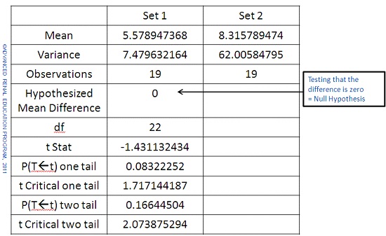
We have the choice to choose a one-tailed or two tailed test: if we do not make any assumption as to whether the mean of set 2 is larger or smaller than that of set 1 then we should chose the 2-tailed test. We see that the p value is 0.166, which is much greater than 0.05 (5% level of significance). The test tells us that there is inadequate evidence to reject the Null Hypothesis and that the means are not significantly different. Note that if we had tested for mean set 2 is larger than mean set 1 then the p value (one-tailed) would be 0.083 which is much nearer to 0.05 but still not significant.

If we add another set, Set 3 which has a mean value very close to that of Set 2, but arrange the set to have a smaller variance we can compare Sets 1 and 3 using the same test. The results are shown below:

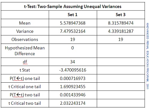
On face value the means look equally different to those in the earlier example. Note, however, that data Set 3 has a much smaller variance than we saw for Set 2. Now we see that the p value (2-tailed) is 0.0014 which is much smaller than 0.05. This tells us that there is only about 1 chance in 1000 that the means are different by random chance. We can reject the Null Hypothesis; the means are significantly different.

If we calculated the 95% confidence intervals (CI) for sets 1 and 2 we find for set 1 (4.36 to 6.8) and for set 2 (4.77 to 11.87). Obviously the 95% CI for set 2 includes most of the values for the CI for set 2 so that there is a greater than 5% chance that the data sets come from the same population. By contrast, the 95% CI for set 3 is (7.38 to 9.26) and does not include the values of the CI of set 1. There is a less than 5% chance that the data of set 1 come from the same population as those of set 3¹.

Comparing Proportions or Distributions

A fairly common problem in clinical practice is that where we seek to compare two populations by the proportions in each that indicate a certain characteristic. An example would be 100 patients randomized to receive either treatment 1 or treatment 2 (50 to each group). Treatment is measured as either success or failure. If Treatment-1 provides 50% success and Treatment-2 65% success, are the two treatments actually different or is this difference due to chance alone?

Again, statistics provides various methods for comparing the two treatments and providing a measure of the true difference. We state the Null Hypothesis that the two treatments are equally effective and test the probability that this is true. The Chi-square (c²) test is one example of a test that would solve the question asked by the above example.

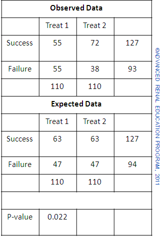
A simple illustration of the test is shown above. First we record the results of the treatments as shown under observed data. For the combined treatments we see that there were 58% successes and 42% failures. We then set up a second table which attributes to each treatment these success and failure rates with the numbers we would have expected if the overall results applied to both treatments; expected data. The Chi-square test is then used to compare the observed results and the expected results and reports a p value. The p value here is 0.11 which is larger than 0.05. The apparently higher success rate for Treatment 2 would occur by chance alone in 11% of trials. The results do not indicate that Treatment 2 is superior to Treatment 1.

In the second example the number of subjects in each group is increased, but the difference in treatment success (increase by 15%) for treatment 2 compared to treatment 1 is proportionately the same. Now we see that the difference is significant with p value 0.022, which is less than 0.05. The reason why the two trials produce differently significant results is similar to that when we compared means above; the additional numbers for this second trial have the effect of reducing the variance of the results and therefore increase the significance of the difference.

The examples here for statistical methods of comparing data and testing whether the difference detected is due to chance alone or is significant, only provide a minimal insight into the possible methods available which are numerous and can be used for very complicated series of data.

   ¹ These confidence intervals are approximations which assume a completely normal distribution. More accurate CI can be calculated from the data.

Resources

Dawson B, Trapp RG. Chapter 8. Research Questions About Relationships among Variables. In: Dawson B, Trapp RG, eds. Basic & Clinical Biostatistics. 4th ed. New York: McGraw-Hill; 2004.

Walters RW, Kier KL. Chapter 8. The Application of Statistical Analysis in the Biomedical Sciences. In: Kier KL, Malone PM, Stanovich JE, eds. Drug Information: A Guide for Pharmacists. 4th ed. New York: McGraw-Hill; 2012.

Godfrey K. Chapter 6. Testing for Relationships, Reporting Association and Correlation Analyses. In: Lang TA, Secic M, eds. How to Report Statistics in Medicine. 2nd ed. Philadelphia: American College of Physicians; 2006.

P/N 101850-01 Rev B 02/2021