In describing measurement of event rates, we refer to the death rate expressed either as a percentage of all patients at risk or as the rate per period risk. These data tell us, for the period measured, how many patients died and how many survived. However, many important research questions cannot be addressed using event rates alone. For example, what about patients who did not die, but stopped treatment (e.g., patients who were transplanted or moved to peritoneal dialysis from hemodialysis treatment)? What is the probability that a patient will die having received treatment for 6 months compared to the probability of death after 6 years of treatment? When comparing two treatments over a period of time, how do we measure the risk of failure (or success) for those who have not yet experienced an event?

To address these problems, statistics offers what are called Life Table Methods. There are several variants of the basic statistic; we will explore two: the Kaplan-Meier probability of survival method and the Cox proportional hazards model.

Kaplan-Meier Probability of Survival

Kaplan-Meier is the most commonly used life-table method in medical practice. It adequately copes with the issues raised above, such as patients for whom the event has not yet occurred and for those lost to follow up. The data required by the method include the time of commencement of the treatment and the time the measured event occurred (e.g., death, relapse, or hospitalization). Patients who dropped out from treatment and those who are still alive at the end of the study period are “censored,” but the contribution that they have made to the event probability are fully accounted for.

In simple terms, what the method does is record the time since initiation of treatment at which an event occurs (e.g., 3 days, 104 days) and counts the number of patients at risk of the event at that time. The rate of the event at that time is then one divided by the number at risk. This is repeated for each event at each time. By multiplying the rate at each time by that for the time of the previous event, a cumulative rate and probability can be calculated. Patients who do not experience the event contribute to the number at risk but not to the event rate for as long as they remain on treatment.

An example of the graphical output of a Kaplan-Meier survival analysis is shown below

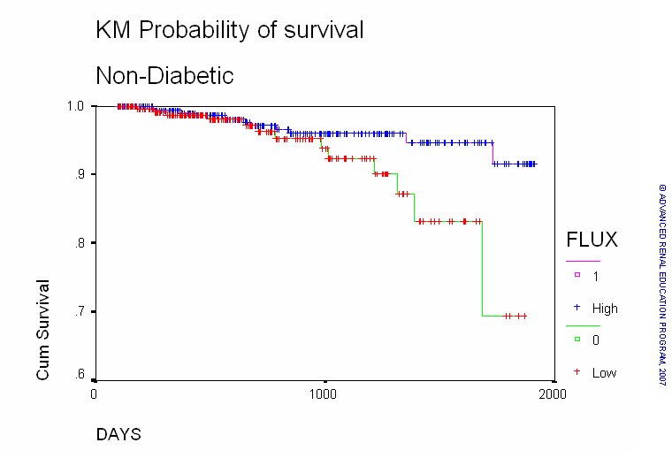
The chart above compares the effect of high-flux dialysis (HFD) to low-flux dialysis (LFD) on patient survival. One of the features of the Kaplan-Meier is the ability to compare different categories of patients or different treatments. Time (days) is seen on the X-axis and the probability of survival on the Y-axis. The points on the chart represent the probability of survival at each interval of time for HFD (upper line) and LFD (lower line).

It is clear that the survival for patients on HFD exceeds that for patients on LFD particularly where survival after about 3 years (1000 days) is concerned. The probability of a patient on HFD surviving 5 years (about 1800 days) exceeds 95%, whereas that for the LFD patients is 0.83 (83%). But is the difference statistically significant? The Kaplan-Meier method provides several statistical tests of significance. The test used in the above analysis (Log Rank test) reported that the p value was 0.03. This means that there is a 3 in 100 probability that the difference is due to chance alone.

Cox Proportional Hazards Model

The Kaplan-Meier method does permit comparisons between patient groups or between different therapies. It cannot, however, be used to measure the impact of a continuous variable (e.g., serum albumin concentration) on the probability of an event, nor can it definitively quantify the risk of the event according to the value of a variable. Cox proportional hazards model is a statistical method that also determines a cumulative probability of an event but also accounts for the impact of other variables upon that probability. The independent variables may be either continuous or discrete. In a sense, the Cox model is a merger of logistic regression and life-table analysis.

The method is too complicated to describe here, and we will confine the discussion to interpretation of the results. As the name of the method suggests, one of its useful functions is the calculation of a hazard ratio (HR) or relative risk (RR). The HR is somewhat similar to, but should not be confused with the odds ratio (OR) described under logistic regression. The HR tells us the degree to which a variable impacts the probability of the event being measured. We can then state the relative risk of the event attributable to the variable.  The most important feature of the Cox model is that the model calculates the hazard effect of each variable while fully accounting for all other variables included in the model.

For example, an analysis was designed to determine whether the composition of a dialyzer membrane had an effect on mortality. During the analysis, standard cellulose membranes were compared to treatment with modified cellulose or synthetic membranes. Since many different patient and treatment variables affect death, it was necessary to build a model which included all of these variables plus the membrane-type variable (i.e., it was necessary to separate the membrane effect from all the other confounding variables). In this model, the authors included factors such as patient age, gender, the presence or absence of diabetes, etc. The model then reports the relative risk of death for all of these factors and for membrane effect. It can then determine whether the factors are acting independently or interdependently on the risk of death. The model also reports the significance level for the effect of each variable.  Like the odds ratio in logistic regression, the significance of the RR attributable to any variable is dependent upon the confidence interval around the value of the RR. A RR above 1 indicates increased risk and values below 1 reduced risk. If the 95% confidence interval includes 1, the effect is not significant.

In this example, the use of modified cellulose or synthetic membranes reduced the risk of death by 18% (RR = 0.82; 1-0.82 = 0.18 x 100%= 18%) when compared to treatment with standard cellulose. The reduced risk was significant (p = 0.002). The results also showed that the risk reduction effect was significant for deaths due to coronary artery disease (CAD: p = 0.007) and deaths due to infection (p = 0.03) but not for deaths due to malignant disease (p > 0.05) or deaths due to cerebrovascular disease (p > 0.05). It is important to note that the reduction in risk of death associated with membrane type is independent of the effect of all the other variables that were entered in the model.

References:

Dawson B, Trapp RG. Chapter 9. Analyzing Research Questions About Survival. In: Dawson B, Trapp RG, eds. Basic & Clinical Biostatistics. 4th ed. New York: McGraw-Hill; 2004.

Glantz, SA. Primer of Biostatistics, Seventh edition. Chapter 11. How to Analyze Survival Data. New York: McGraw Hill; 2012.

Walters RW, Kier KL. Chapter 8. The Application of Statistical Analysis in the Biomedical Sciences. In: Kier KL, Malone PM, Stanovich JE, eds. Drug Information: A Guide for Pharmacists. 4th ed. New York: McGraw-Hill; 2012.

 

P/N 101853-01 Rev B 02/2021