For the discussion of this topic, let us use an example where one hundred hypertensive patients are prescribed an antihypertensive agent. To assess the efficacy of the treatment, BP recordings are taken before and after treatment. One way of reporting the effectiveness of the treatment would be to list all subjects’ BPs before and after treatment in a table. It would obviously be extremely difficult for an observer to assess whether the treatment had been successful. Summing all the BP values before treatment and dividing by the number of observations would provide an average value for the pre-treatment BP; the same could be done for post-treatment. Instead of long lists we would only have to compare two values. The averages pre- and post-treatment could then be compared and an assessment made as to whether the difference was meaningful.

Mean and Median

In general, “the average” is expressed in statistical terms by either the mean or the median (there are other measures of center which we can ignore for now). The mean is the arithmetical average – the sum of all values divided by the number of observations. The median is that value which separates the upper 50% of subjects from the lower 50%. To understand the difference between mean and median we have to first examine the concept of normality of distribution.

Figure 1. The distribution of body weights of over 700 dialysis patients (bars) and the cumulative percentage frequency (line)

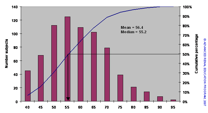
Figure 1 shows a histogram of the distribution of body weights of over 700 dialysis patients (bars) and the cumulative percentage frequency (line). Imagining a line drawn through the upper points of the bars would produce a “bell shaped” curve; data that have this sort or distribution are called normal distributions. We can calculate the mean (sum of all values divided by the number of observations) and find the value 56.4 kg. To find the median we determine the value for weight that divides the population into two equal halves as shown by the arrow dropping from the cumulative frequency line; the actual value is 55.2 kg. Typically, for such normally distributed data the median and mean are very similar.

Figure 2. The population from above including a small number of patients with high body weights.

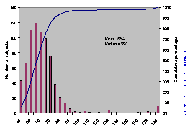
In Figure 2 the population is almost the same but includes a small number of patients with extremely high body weights.

Again, we can estimate the mean and median weights. The addition of the heavier patients, although few in number, has a significant effect to increase the mean weight (by 3 kg) but has little effect on the median. The median is little affected by extreme outliers whereas the mean is sensitive to them. Knowledge of how a data set is distributed indicates which measure of center is more appropriate.

Dispersion about the center¹

Although measures of center provide useful summary information about a data set, they tell us nothing about how the data are dispersed. One way of indicating data dispersion would be to report the range of data values – lowest and highest. In Figure 1 the weights range from 19.94 to 94.8 kg so the data set could be summarized by reporting the median and the range as 55.2 (range: 19.4‑94.8). For the data set in Figure 2 the report would be 55.8 (range: 19.94-180).

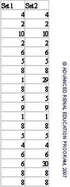
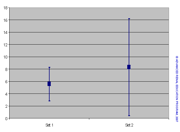
Other measures of dispersion are the variance and the standard deviation (SD: = √variance). The variance and SD are calculated from standard statistical formulas. To illustrate this we will use two sets of data as shown in the table.

The data sets are quite similar except that Set 2 includes 2 more extreme values. We can see the effect of these differences by expressing the mean, variance and standard deviations for the two series:

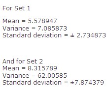
Note the ± sign before the SD; this indicates the dispersion of values above and below the mean.

The larger variance and standard deviation of Set 2 indicate greater dispersion of the data around the mean than for Set 1. Variance is very important when comparing the means of two or more data sets. The means and SD are shown in graphical form in Figure 3.

Resources:

Dawson B, Trapp RG. Chapter 8. Research Questions About Relationships among Variables. In: Dawson B, Trapp RG, eds. Basic & Clinical Biostatistics. 4th ed. New York: McGraw-Hill; 2004.

Walters RW, Kier KL. Chapter 8. The Application of Statistical Analysis in the Biomedical Sciences. In: Kier KL, Malone PM, Stanovich JE, eds. Drug Information: A Guide for Pharmacists. 4th ed. New York: McGraw-Hill; 2012.

Godfrey K. Chapter 6. Testing for Relationships, Reporting Association and Correlation Analyses. In: Lang TA, Secic M, eds. How to Report Statistics in Medicine. 2nd ed. Philadelphia: American College of Physicians; 2006.

 

P/N 101880-01 Rev B 02/2021