Regression is similar to correlation and the two are often confused. Regression analyses are used to predict the value of one variable based on knowledge of another. Specifically, regression seeks to build a mathematical model that allows the value of one or more dependent (response) variables to be predicted for a particular independent (explanatory or stimulus) variable.

The regression models range from simple univariate (one stimulus and one response) to multiple (one or more responses to more than one stimulus). Linear regression models are those where the response changes in a linear fashion. Responses to stimuli, however, may not follow a linear path but may show a curvilinear pattern or even a parabolic (U shaped) pattern. In some cases the plot of the raw stimulus and response data shows a curvilinear shape, but transformation of one or both data sets can convert the relationship to linear (e.g., log transformation) relationship.

Simple Linear Regression

For example, in a hemodialysis unit, a clinician may be is interested in predicting the fall in systolic BP (SBP) during the first hour of dialysis according to the applied ultrafiltration rate (UFR). The change in SBP and UFR are recorded during 33-dialysis sessions. The data are then plotted as a scatter chart as seen below.

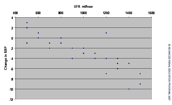
Based on the scatter plot, there appears to be a negative (inverse) relationship: As the rate of UF increases, SBP falls (i.e., becomes more negative). Using correlation statistics we can confirm this relationship. However, our main interest is to be able to predict the degree of fall of SBP in response to UF. By a method called least squares analysis, we can plot a line through the points on the graph that would best fit the data. This is similar to finding the “mean” for the SBP response at each UFR. The derived line is shown in the chart below. This line can be expressed mathematically by the formula Y = bX + a where ‘a’ is the imaginary or real value of Y when X=0 ([Y=b*0 + a] = [Y=a]). ‘b’ is called the regression coefficient, which is slope of the best-fit line. Specifically, ‘b’ represents the amount of change in Y for each unit of change in X. If ‘b’ is negative, Y falls for each unit rise in X; if ‘b’ is positive, Y rises for each unit increase in X.

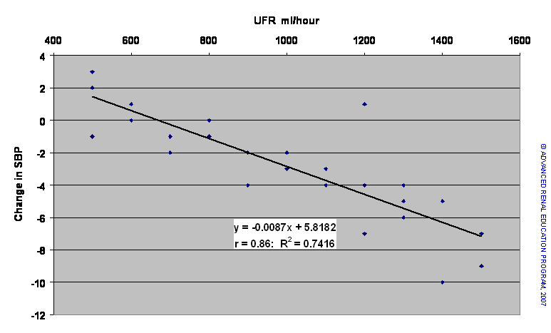
The line in the chart above has the equation Y = -0.0087X + 5.82 (where Y = change in SBP mmHg and X = UFR ml/hour). This linear regression model predicts that for each increase in UFR by 100 ml/hour, the SBP will fall by 0.87 mmHg (100*0.0087 = 0.87). The correlation coefficient r = -0.86 suggests that the model fits the data quite well. Statistics also provides additional methods to test the “goodness of the fit” of the model; which we need not explore here. Furthermore, the coefficient of association R² = 0.74 tells us that 74% of the change in SBP is actually due to the change in UFR and 26% is due to some other effect not definable in this study.

Non-linear regression

When plotted data do not assume a linear relationship, it is useful to replot the data with one or both sets of values transformed. Various transformations can be tried (e.g., using log transformation, invert values, power values, etc.) and experience usually informs which will work best. The results of the regression model can then be converted back to the normal value to derive the predictions required. However, some data are not linear and cannot be converted even with transformation. An example is shown below.

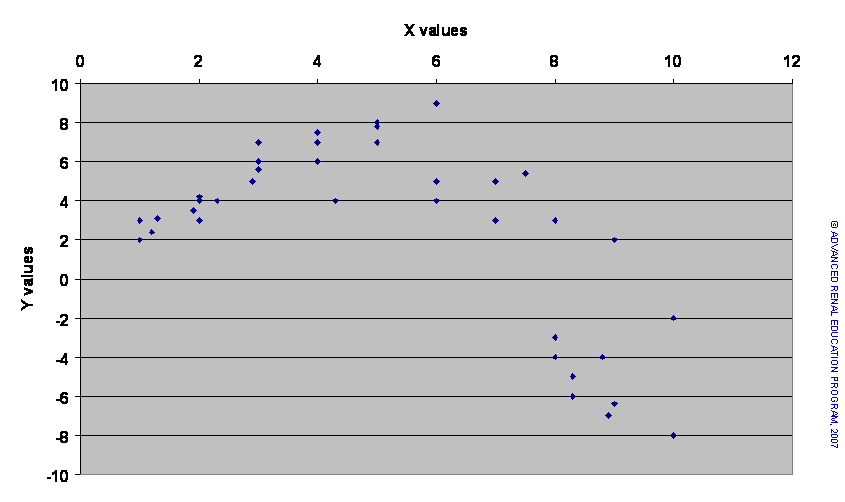
The X values in the scatter plot above represent the dose of an agent known to stimulate a metabolic function, which is indicated by the Y values. The relationship is obviously not linear. In fact, initially, increasing dose of X enhances the Y response; however, above a certain dose of X the Y response seems to be inhibited. It is possible to model this non-linear regression, although there are many hazards in building such models.

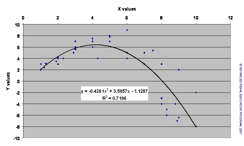
One such model is shown in the chart above as a polynomial function. The R² value for the fitted regression suggests a good fit but this would need to be stringently tested by appropriate statistical methods.

Logistic regression

How can we model regression when the response variable is categorical (yes/no: on/off) rather than continuous? Examples include the following: Death in response to categorical or continuous independent variables. Does being diabetic (yes/no) affect the mortality of dialysis patients? Does the dose of delivered dialysis (Kt/V – a continuous numerical variable) affect death rate? It would be possible to measure death rates in diabetic and non-diabetic patients and compare the results to indicate an effect, but such a method would not permit the meaningful prediction of the effect of diabetes on death.

To develop a statistical model that enables the quantifiable prediction of the effect of a variable on a categorical event, one utilizes a technique called Logistic Regression. The mathematics is more complex and need not be developed here. The output of logistic regression models are usually expressed as the odds ratio that the categorical event will occur according to the value of the dependent variable (if a continuous variable with a numeric scale) or whether the dependent categorical covariate is present.

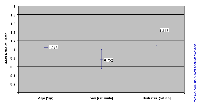
An example of a logistic regression analysis is shown above. The graph depicts the impact of various demographic factors and laboratory results on the death of PD patients in the USA. Only three covariates are shown here: age, patient sex and diabetes. Age is a continuous variable measured in years. Sex is a categorical variable, male or female, and diabetes is a categorical variable. Note the way the data are presented: each data point is a horizontal bar with a vertical line extending above and below the data point. This looks like the mean and SD results shown in Figure 3 but is not. The vertical bar represents what is known as the confidence interval for the odds ratio.

If the odds ratio (OR) is greater than 1 the effect of an increased value of the variable or the presence of the covariate is to increase the probability of the event (death in this case); if less than 1 the effect is to reduce the event probability. The nearer the OR to the value 1 the less the effect; an OR of 1 indicates no effect. The statistic reports the OR and a confidence interval (CI) for the OR. For example, for diabetes in the above example, the OR is 1.44 and the 95% confidence interval is 1.09 to 1.9. Stated another way, the estimated odds ratio of death for diabetics compared to non-diabetics is 1.44, and there is 95% certainty that the actual OR lies somewhere between 1.09 and 1.9. It should be apparent that if the 95% CI includes the value 1 then there is a chance that there is no effect. We can therefore state that if the CI for the OR includes the value 1 the detected effect is not significant.

The figure above shows that for each 1-year additional age the OR of death is 1.043. The confidence interval (1.032 to 1.055) does not include 1; the vertical bar does not cross the line for the value 1. Another way of expressing this would be to state that for each additional 1-year of age, the odds of dying are increased by 4.3% (1.043 = 1 + 0.043: 0.043 = 4.3%).  Females (compared to males) have a 25% reduced odds of dying (1 – 0.75 = 0.25 x 100% = 25%; note, however, that the upper part of the CI bar comes very close to 1 (actual CI = 0.56 to 0.99) so that the significance of this OR is lower. On the other hand, having diabetes increases the odds of dying by 44% (OR = 1.44) and the vertical bar of the CI is distant from 1.

Logistic regression also builds a predictive model for the event incorporating those variables and covariates that have a statistical significance. The model equation has the basic form Y = bx + a  that we saw earlier for linear regression. In the example from Figure 8 there are three variables, so that the model would actually look like this: Y = b₁x₁ + b₂x₂ + b₃x₃ + a. With the values for the three coefficients, b_{1 to 3}, we could predict the combined effect of the three variables on death odds. Moreover, the statistical method would provide measures of goodness-of-fit for the model.

Resources:

Dawson B, Trapp RG. Chapter 8. Research Questions About Relationships among Variables. In: Dawson B, Trapp RG, eds. Basic & Clinical Biostatistics. 4th ed. New York: McGraw-Hill; 2004.

Walters RW, Kier KL. Chapter 8. The Application of Statistical Analysis in the Biomedical Sciences. In: Kier KL, Malone PM, Stanovich JE, eds. Drug Information: A Guide for Pharmacists. 4th ed. New York: McGraw-Hill; 2012.

Godfrey K. Chapter 6. Testing for Relationships, Reporting Association and Correlation Analyses. In: Lang TA, Secic M, eds. How to Report Statistics in Medicine. 2nd ed. Philadelphia: American College of Physicians; 2006.

 

P/N 101852-01 Rev B 02/2021